Filtering Rows

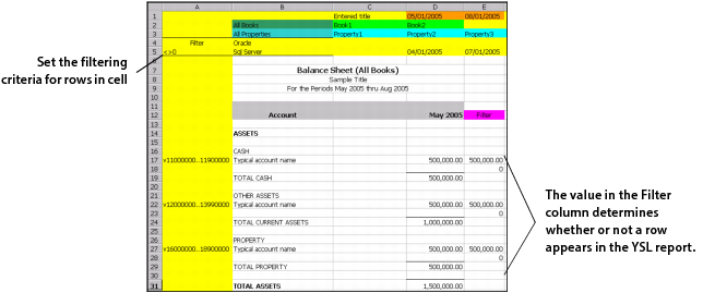
Each YSL worksheet template must include a filter column, typically the column furthest to the right on the spreadsheet. Enter the word Filter (case insensitive) into a column cell to designate that column as the filter column of the YSL report. At run time, YSL “filters” the rows of a YSL report by comparing the value in each filter column cell with the filtering criteria entered in cell A5. The value in the filter column determines whether or not a row appears in the YSL report.

Column A must not be the Filter column, and the keyword Filter is always placed in a row greater than Row 6.

In the previous example, the condition for displaying a row is set to <>0 (not zero). This means that a row is included in the YSL report if the value in the filter column is not equal to zero. At run time, the YSL report appears as follows:

Note that all the rows that have filter column values not equal to zero (a logical test, as defined in cell A5) are included in the Balance Sheet YSL report. (This example's filter column is viewable, but you would normally hide this column on your YSL reports.)

An alternative example might be to set the row filtering conditions in cell A5 to >10000000. In this case, only the rows with sums greater than ten million are included in the YSL report.

The conditions you set for filtering rows are based on your specific needs.